System Identification and Position Control of a Linear Motor (part 1)
Table of contents
- 1- Description
- 2- Deriving system’s dynamic equations
- 3- Getting System Parameters Experimentally
- 4- Adding PI position controller
In this post, I will share a project I worked on for the Advanced Control course during my master’s at AUS. Group members:
- Ehab Al-Khatib,
- Wasim Al-masri,
- and myself.
1- Description
The aim of the project is to identify a mechanical-electrical system. The system in hand is a linear voice coil motor. A PI controller for the position was later added and comparison is made between real system response and simulated response . The most important paramter to estimate is friction (other paramters are either given ex: motor force constant, or easy to measure, ex: coil resistance).
Firiction acts in the opposite direction of the motion and has three components:
-
Stiction: is the static force, the force which the motor needs to overcome in order to move the mass. We are interested to model the system during motion so we will ignore this value.
-
Coulomb friction: A constant force (opposite to motion).
-
Viscous friction: firction force propotional to speed (i.e. \(\propto \dot{x}\)).
Coulomb friction and viscous friction are estimated using curve fitting. By fitting actual system response (obtained experimentally) to system mathematica model. The second phase (part 2 of the post) is to estimate friction components using a state observer. The value of the estimated friction is used to add a friction compensator to the PI position controller.
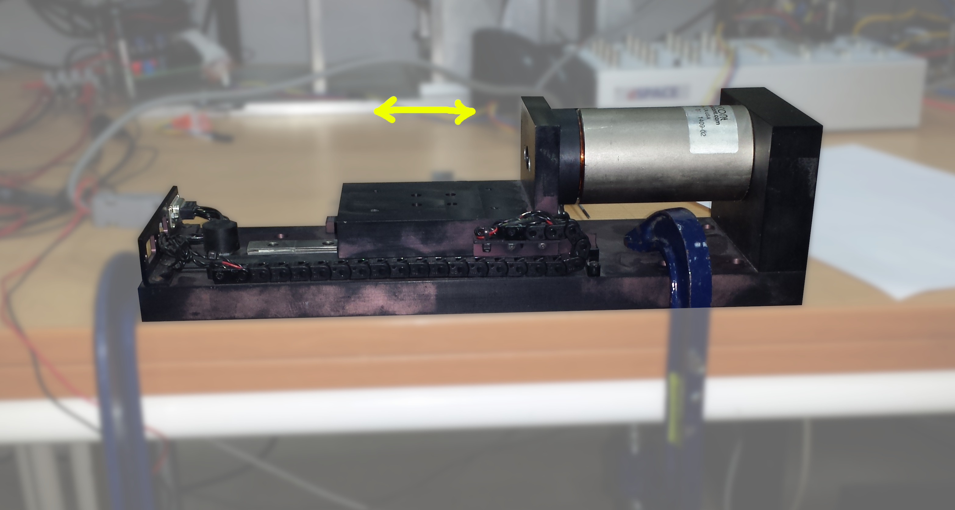
2- Deriving system’s dynamic equations
A) Horizontally oriented

Where \(K_F\) is the force constant of the motor (given in the datasheet), and \(i(t)\) is calculated from the input voltage \(v_a\) using the model of the electrical part of the motor:
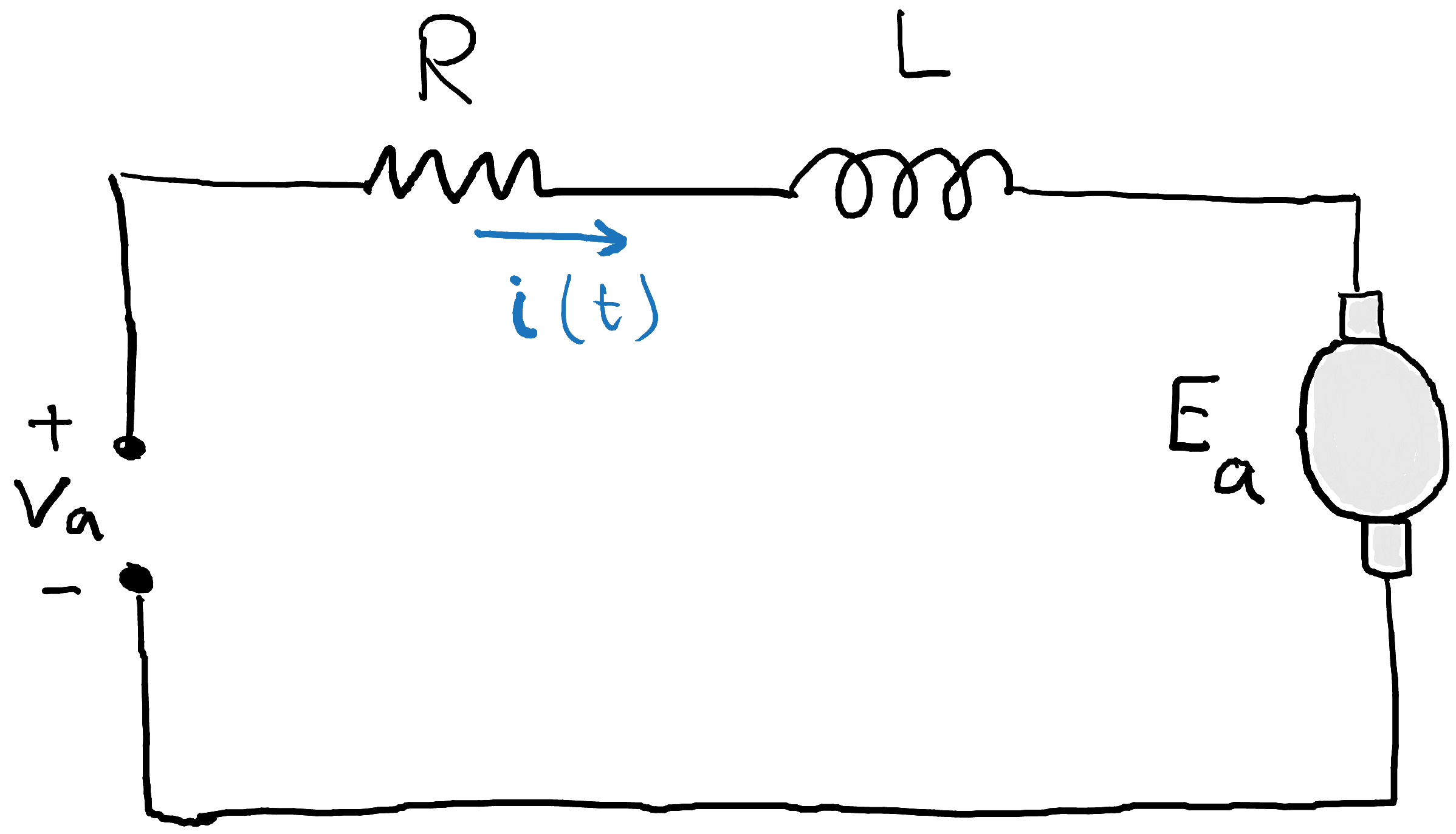
Where \(K_{emf}\) is the back EMF constant, \(R\) is the coil resistance and \(L\) is the coil inductance, which are all given in the motor datasheet.
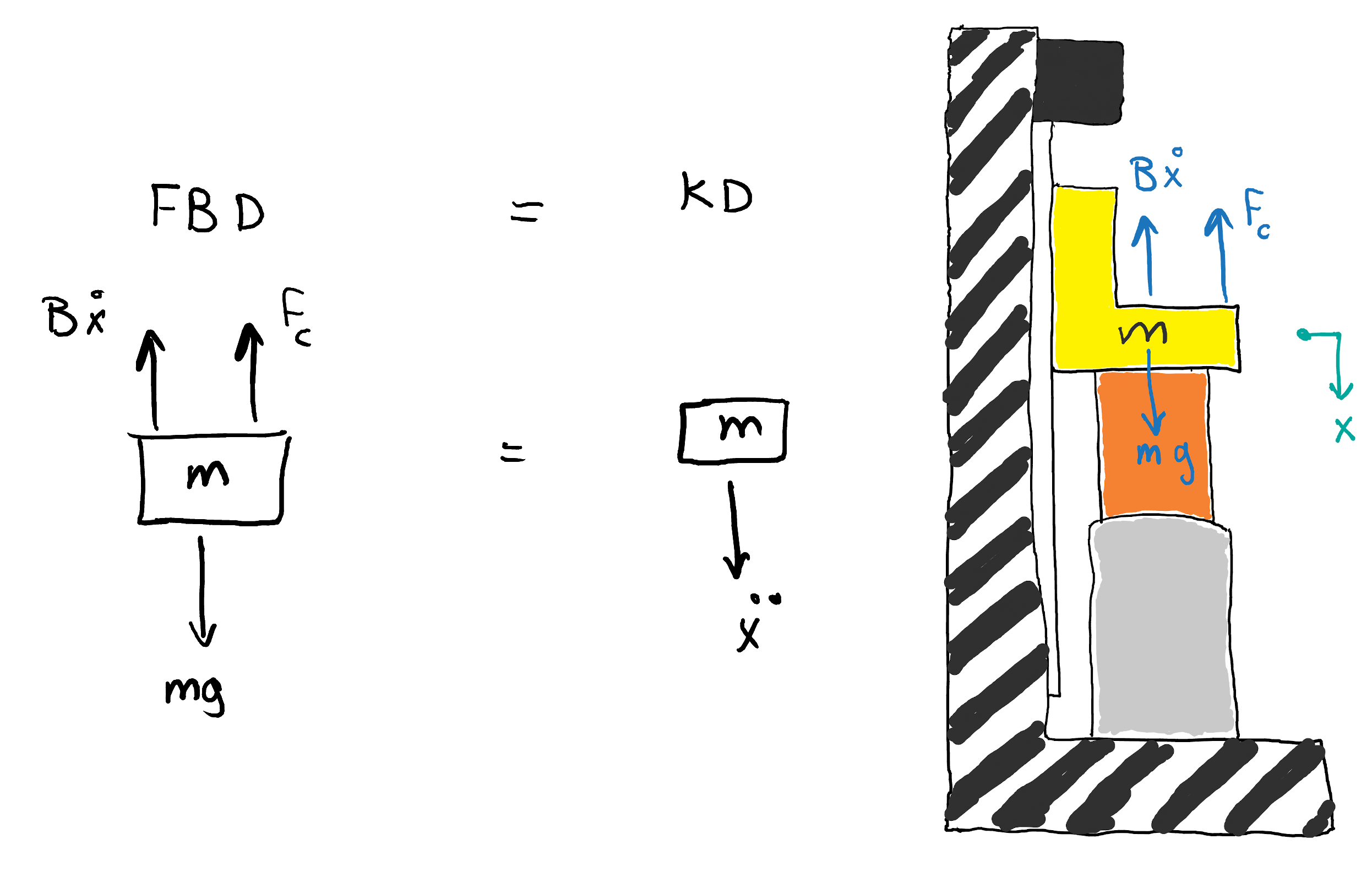
B) Vertically oriented (setup used for system identification)
3- Getting System Parameters Experimentally
A) Actual system response
The setup is fixed vertically and in each experiment the mass is lifted around \(2 ~cm\) upward (this will be the reference point, i.e. \(x = 0\)), then released. The motion of the mass is recorded using an encoder. This was repeated multiple times, and the average of these runs was computed:

Now that we have the actual system response. We need to solve the ODE in equation \((3)\) and find a time-domain solution (theortical system response). Which will then be used in the curve fitting step.
B) ODE solution
\(m ~\ddot{x} = mg - F_c - B ~\dot{x} ~~~~~~~(3)\)
- Homogenous solution
It’s a \(1^{st}\) order linear ODE. We can assume the solution to be \(v(t) = c ~e^{\lambda ~t}\). Plugging the solution back into the ODE, we find \(\lambda\). By doing that we get the homogenous solution \(v_h(t)\):
\[v_h(t) = c ~e^{-{B \over m} ~t}\]- Particular solution
Substitute in the ODE, we get:
\[B ~.~ k = mg - F_c\] \[k = {mg - F_c \over B}\]Applying initial condition \(v(0) = 0\):
\[v(t) = -\bigg({mg - F_c \over B}\bigg) ~e^{-{B \over m} ~t} + {mg - F_c \over B} ~~~~~~~~(4)\]By integrating, and applying the initial condition \(x(0) = 0\), we get:
\[x(t) = \bigg({m^2g - m ~ F_c \over B^2}\bigg) \bigg( e^{-{B \over m} ~t} ~+ ~{B \over m} ~t ~- ~1 \bigg)\] \[x(t) = c_1 \bigg( e^{-c_2 ~t} ~+ ~{1 \over c_2} ~t ~- ~1 \bigg) ~~~~~~~~(5)\]Where:
\[c_1 = {m^2g - m ~ F_c \over B^2}\\ c_2 = {B \over m}\]By fitting equation \((5)\) on the actual response data, we obtain \(c_1\) and \(c_2\). This gives us two equations, if mass is known, we can solve for coulomb friction \(F_c\) and viscous friction coefficient \(B\).
We were not allowed to disassemble the motor, take the mass out, and measure it on a scale. Luckily, the mass was given in the datasheet. However, in the following step, we will also find it experimentally and also find upper and lower bounds on the coulomb friction \(F_c\) which can help in the curve fitting step.
Note: velocity equation can also be used for curve fitting and finding parameters, but velocity data had more noise that position data (as expected due to differentation, i.e. \(v(t) = {dx(t) \over dt}\)).
C) Pre-curve fitting step and getting the mass
Since Coulomb friction force \(<\) stiction force, estimating stiction gives us an upper bound on \(F_c\).
- Finding stiction
When the setup is horizontally oriented, and when the mass is motionless and under equilibrium, only two forces are acting on the mass and they are equal in magnitude but opposite in direction:

\(K_F\) is given in the datasheet and \(= 10.1 ~({N \over A})\). By increasing motor current (increaing \(F_m\)) until we reach an equilibrium point (just before the mass start to move), we find the stiction:
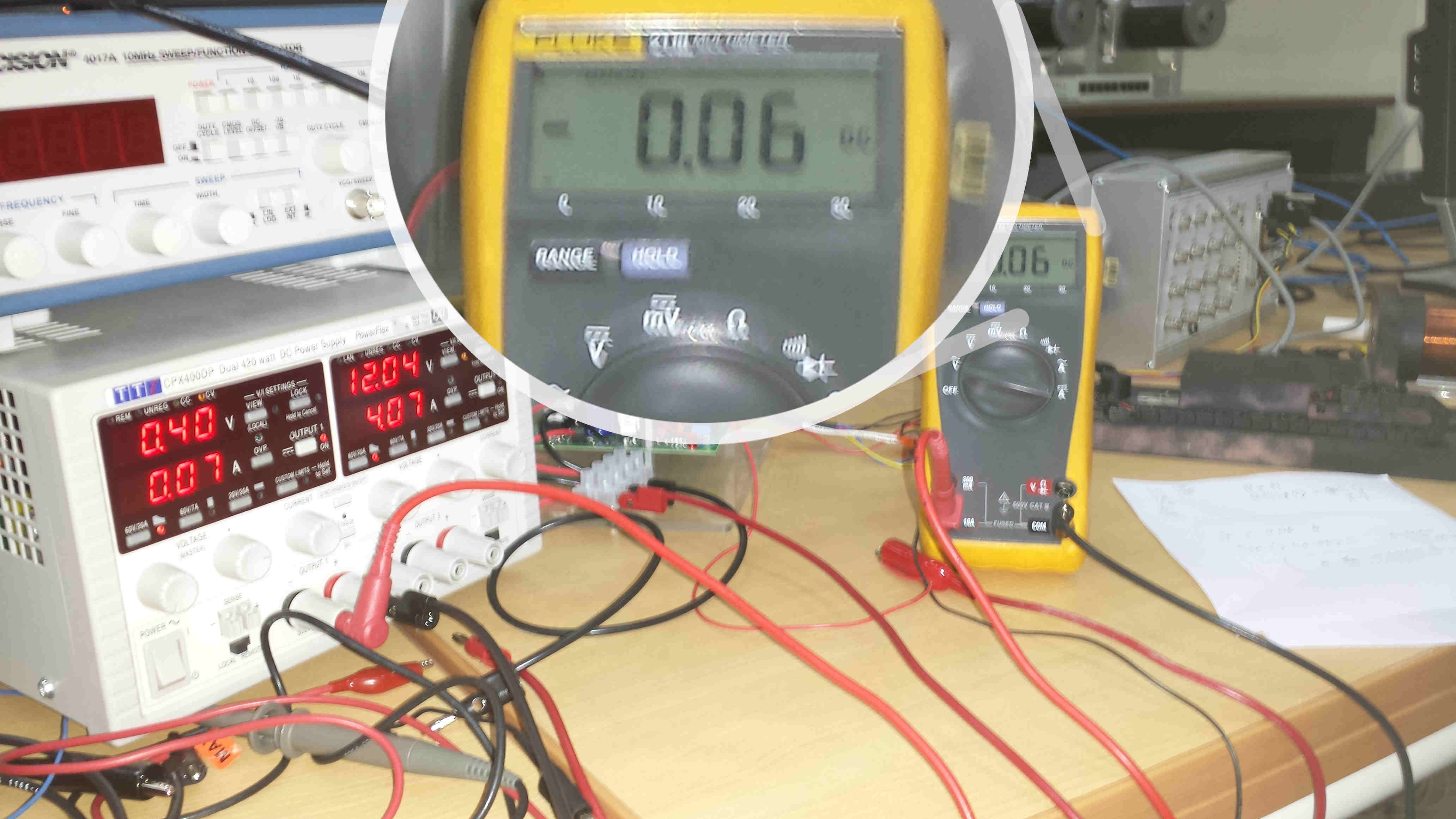
From that we conclude the upper/lower bounds of \(F_c\):
\[0 < F_c < 0.606\]- Finding mass
When the setup is vertically oriented, and during equilibrium with no motion at all, only three forces are acting: the weight (unknown), motor force, and stiction (known from previous step).
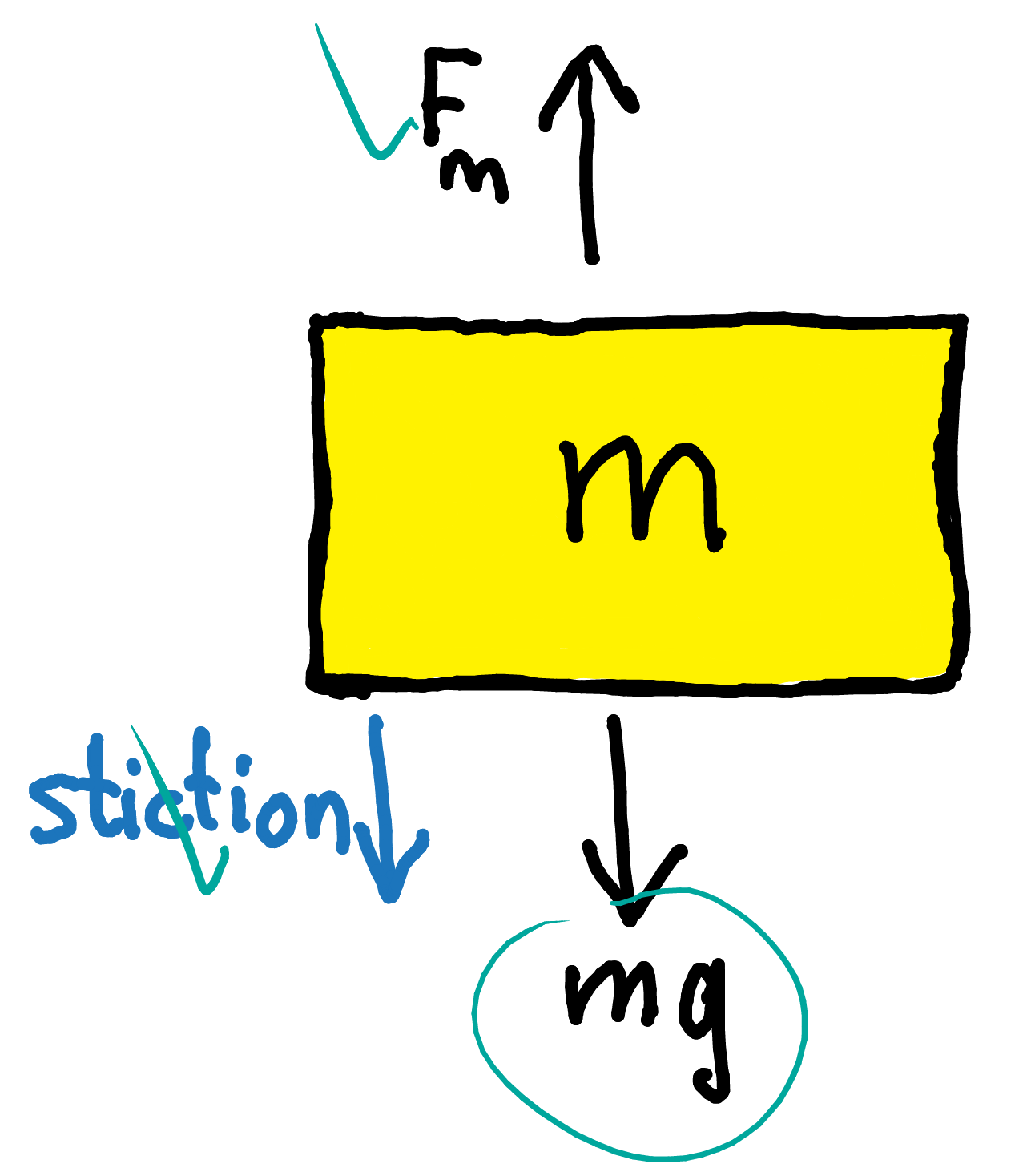
Mass was found to be:
\[m = 797.9 ≈ 800 ~grams\]D) Curve fitting
Using Matlab curve fitting toolbox and applying the lower and upper limits (discussed previously), the following results were obtained. Note that, the range that bounds the viscous friction \(B~\dot{x}\) is also known since it can’t be larger than the weight and it should be positive.
\[F_c = 0.5067 ~~(N)\\ B = 5.826 ~~({N \over m/s})\]4- Adding PI position controller
A PI controller is used with the same gains for both simulated and real systems, the responses are then captured and compared. System response characteristics (overshoot, settling time) are not specified. So,the PI gains have been manually tuned until system response was satisfactory. The assigned gains were:
\[K_p = 25\\ K_I = 7\]The figure below is the real and simulated closed loop system response with a step input of \(3 ~cm\):
In the next post, we will estimate friction components using a state observer. And them to add a compensator to the PI controller

